分组摘要
摘要函数summaize()结合分组函数group_by()能够很方便地得到统计结果。
结合使用管道符号%>%,可以省却很多变量命名的麻烦,使代码更加简洁。
 1
 2
 3
 4
 5
 6
 7
 8
 9
10
11
12
13
14
|
# 分组,摘要,结果过滤一步完成
delays <- flights %>%
group_by(dest) %>%
summarise(
count = n(),
dist = mean(distance, na.rm = TRUE),
delay = mean(arr_delay, na.rm = TRUE)
) %>%
filter(count > 20, dest != "HNL")
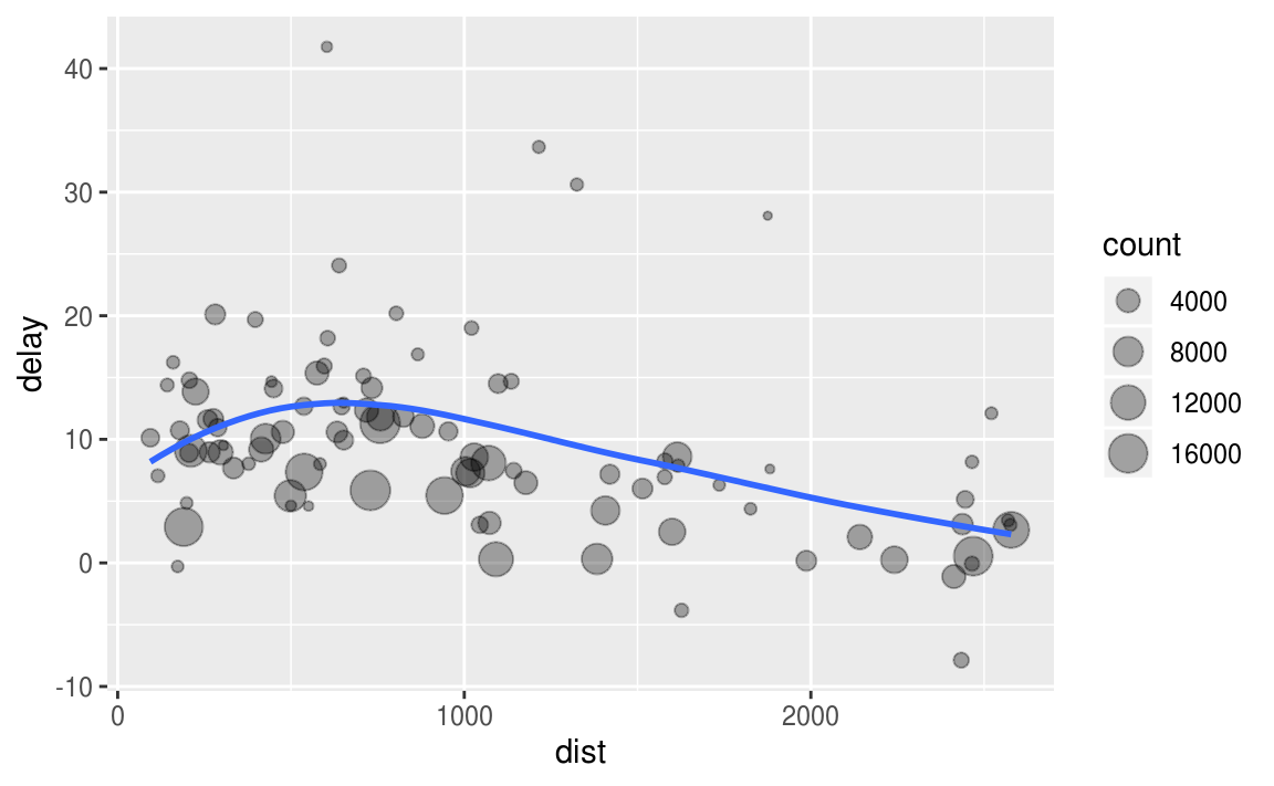
ggplot(data = delay, mapping = aes(x = dist, y = delay)) +
geom_point(aes(size = count), alpha = 1/3) +
geom_smooth(se = FALSE)
#> `geom_smooth()` using method = 'loess' and formula 'y ~ x'
|
计数
在整合数据时,使用计数函数n()或计数所有非缺失值sum(is.na(x))常常很有帮助。这使得我们能够查看数据是否来自一些非常小的样本。
 1
 2
 3
 4
 5
 6
 7
 8
 9
10
11
|
not_cancelled <- flights %>%
  filter(!is.na(dep_delay), !is.na(arr_delay))
# 按照航班机尾编号进行分组
delays <- not_cancelled %>%
  group_by(tailnum) %>%
  summarise(
    delay = mean(arr_delay)
  )

ggplot(data = delays, mapping = aes(x = delay)) +
  geom_freqpoly(binwidth = 10)
|
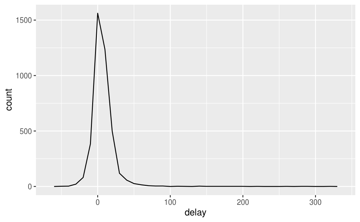
有一些航班的延误时间长达300 min,这是我们需要查看一下样本数量,排除偶然偏差的影响。
绘制一个航班数量对平均延误时间的散点图能够帮助我们直观地理解
1
2
3
4
5
6
7
8
9
|
delays <- not_cancelled %>%
  group_by(tailnum) %>%
  summarise(
    delay = mean(arr_delay, na.rm = TRUE),
    n = n()
  )

ggplot(data = delays, mapping = aes(x = n, y = delay)) +
  geom_point(alpha = 1/10)
|
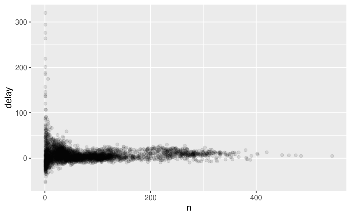
可以见到,在样本数量较少时,平均延误时间的偏差很大。
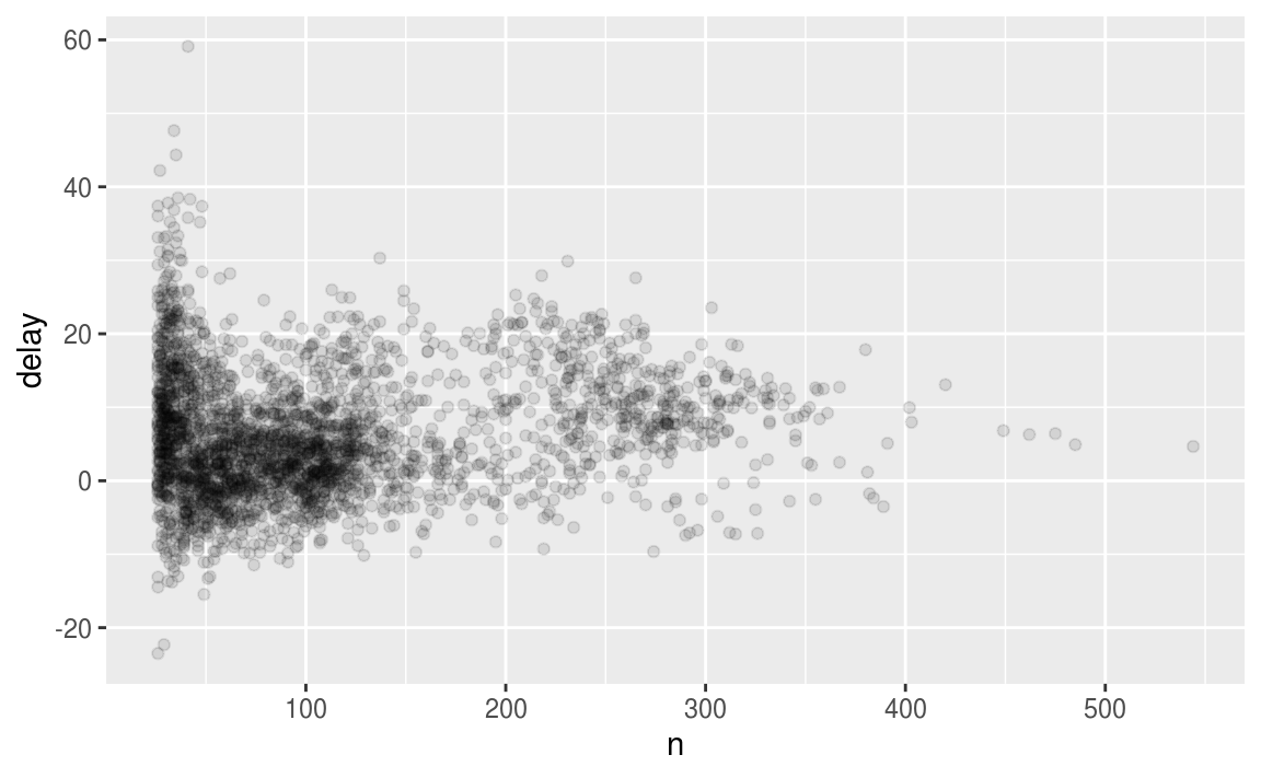
这种情况下,过滤掉最小的哪些观察值能够帮助我们发现规律。
1
2
3
4
|
delays %>%
  filter(n > 25) %>%
  ggplot(mapping = aes(x = n, y = delay)) +
    geom_point(alpha = 1/10)
|
常用的摘要函数
-
位置度量
mean(x)
median(x)
-
分散程度度量
sd(x), 标准差
IQR(x), 四分位距
mad(x), 绝对中位差
-
秩的度量
min(x), quantile(x, 0.25), max(x)
-
定位度量
first(x), nth(x, 2), last(x)
1
2
3
4
5
6
|
not_cancelled %>%
  group_by(year, month, day) %>%
  summarise(
    first_dep = first(dep_time),
    last_dep = last(dep_time)
  )
|
-
计数
n()不需要任何参数,返回当前分组的大小
sum(is.na(x))统计非缺失值的数量
n_distinct(x)计算唯一值的数量
-
逻辑值的计数和比例
sum(x > 10)和mean(y == 0)
按多个变量分组
当使用多个变量分组时,每次摘要统计会消耗一个分组变量。
 1
 2
 3
 4
 5
 6
 7
 8
 9
10
11
12
13
14
15
16
17
18
19
20
21
22
23
24
25
26
27
28
29
30
|
daily <- group_by(flights, year, month, day)
(per_day   <- summarise(daily, flights = n()))
#> # A tibble: 365 x 4
#> # Groups:   year, month [?]
#>    year month   day flights
#>   <int> <int> <int>   <int>
#> 1  2013     1     1     842
#> 2  2013     1     2     943
#> 3  2013     1     3     914
#> 4  2013     1     4     915
#> 5  2013     1     5     720
#> 6  2013     1     6     832
#> # … with 359 more rows
(per_month <- summarise(per_day, flights = sum(flights)))
#> # A tibble: 12 x 3
#> # Groups:   year [?]
#>    year month flights
#>   <int> <int>   <int>
#> 1  2013     1   27004
#> 2  2013     2   24951
#> 3  2013     3   28834
#> 4  2013     4   28330
#> 5  2013     5   28796
#> 6  2013     6   28243
#> # … with 6 more rows
(per_year  <- summarise(per_month, flights = sum(flights)))
#> # A tibble: 1 x 2
#>    year flights
#>   <int>   <int>
#> 1  2013  336776
|
取消分组
ungroup()
参考来源
https://r4ds.had.co.nz/transform.html#grouped-summaries-with-summarise
 次阅读
次阅读